Studio della cinematica degli spezzatori idraulici per roccia

4.1 Caratteristiche cinematiche e coefficiente caratteristico α

Questa sezione studia principalmente la natura geometrica e le caratteristiche del moto del pistone del frantumatore idraulico per roccia, in modo che il moto del pistone diventi più razionale e avvenga secondo il modello di movimento da noi specificato, ottenendo così i migliori risultati di movimento.

Per studiare la cinematica del pistone del frantumatore idraulico per roccia, devono essere chiaramente stabiliti due requisiti:

(1) Deve essere garantita la velocità del pistone all’istante dell’urto sulla coda dello scalpello, affinché raggiunga la velocità massima specificata v _m . In altri termini, nello studio della cinematica, v _m è una costante; indipendentemente dal modello di moto seguito dal pistone, la sua velocità all’istante dell’urto sulla coda dello scalpello deve corrispondere alla velocità massima specificata v _m . Solo in questo modo il frantumatore idraulico per roccia può raggiungere l’energia d’urto richiesta. A _H .

(2) Il ciclo di moto del pistone T è anch’esso una costante, garantendo così la frequenza d’urto f _H del frantumatore idraulico per roccia.

La Fig. 4-1 mostra il diagramma della velocità di lavoro lineare del pistone. Il punto M ha coordinate ( v _m , 0); il punto E ha coordinate (0, T ); il punto N ha coordinate (− v _m , T ). Collegando i punti M e E si forma il triangolo △MOE nel sistema di coordinate v –t , i cui due cateti sono rispettivamente la velocità massima del moto del pistone verso il punto d’impatto e il ciclo di moto del pistone T . Considerando un qualsiasi punto P (v _mo , T ₂^′) sulla linea Me , e collegando PO e PN, quindi PN interseca l' t -asse in K . Il punto K sull'asse del tempo divide il ciclo di movimento del pistone T in due parti: T ₁e T ₂. Chiaramente T ₁ + T ₂ = T , formando due triangoli △OPK e △ENK.

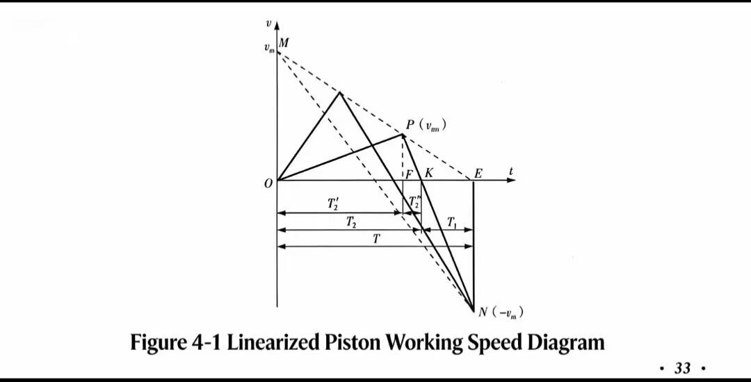
È facile dimostrare che le aree di questi due triangoli sono uguali, cioè △OPK = △ENK, da cui si ottiene v _mo T ₂/ 2 = v _m T ₁/ 2. Chiaramente, nel v –t diagramma, l'area racchiusa dal triangolo △OPK corrisponde alla corsa di ritorno del pistone, mentre l'area racchiusa dal triangolo △ENK corrisponde alla corsa di lavoro del pistone. La corsa di lavoro è uguale alla corsa di ritorno — questo è un dato. In altre parole, la curva O –P –K rappresenta la variazione della velocità del pistone durante la corsa di ritorno; la curva K –N –E rappresenta la variazione della velocità del pistone durante la corsa di lavoro.

Curva O –P –K –N –E rappresenta la variazione della velocità del pistone durante il ciclo di movimento T . Il pistone inizia la corsa di ritorno dal punto d’urto O dove ha contattato la coda dello scalpello, accelerando da v = 0 fino al punto P — commutazione della valvola (quando la velocità del pistone raggiunge la velocità massima della corsa di ritorno v _mo ) — il pistone inizia a decelerare e la sua velocità diminuisce progressivamente fino a v = 0, raggiungendo il punto morto superiore (fine della corsa di ritorno). Il pistone inizia quindi l’accelerazione della corsa di potenza; quando la velocità aumenta fino a v = v _m , colpisce esattamente la coda dello scalpello e la velocità scende immediatamente a zero ( v = 0), e il pistone ritorna al punto di partenza del suo moto, completando un ciclo.

Va sottolineato che, quando la velocità massima e il ciclo del pistone del frantumatore idraulico per roccia sono entrambi fissati, la velocità massima di ritorno v _mo deve necessariamente giacere sulla M –E linea ausiliaria, ovvero nel punto P . Si può immaginare che esistano infiniti punti P sulla linea M –E , il che significa infinite velocità massime di ritorno v _mo , ovvero infinite curve di moto del pistone — il pistone ha quindi infinite modalità di moto tra cui scegliere. Dovremo naturalmente selezionare la modalità di moto ottimale. Questo costituisce il problema di progettazione ottimale oggetto di studio nei capitoli successivi.

Un'analisi più approfondita del moto del pistone può essere effettuata esaminando la Fig. 4-1. A tal fine, dai triangoli simili △MOE e △PFE si ottiene:

v _m / v _mo = T \/ ( T ₁ + T ₂^″) (4.1)

Dai triangoli simili △PFK e △ENK:

v _m / v _mo = T ₁ / T ₂^″                                                                   (4.2)

Pertanto:

T \/ ( T ₁ + T ₂^″) = T ₁ / T ₂^″                                                           (4.3)

Dopo aver riordinato:

T ₁ / T = v _mo \/ ( v _m + v _mo ) (4.4)

Dall’Eq. (4.1) risulta chiaramente che, fissato il ciclo di moto del pistone T e la velocità massima v _m , i cosiddetti diversi schemi di moto presentano curve diverse di variazione della velocità; la caratteristica distintiva è espressa da differenti valori della velocità massima nella corsa di ritorno v _mo e del tempo di corsa di lavoro T ₁. Pertanto, questi due parametri racchiudono la proprietà di caratterizzare le caratteristiche cinematiche di un particolare frantumatore idraulico per roccia.

Tuttavia, il nostro obiettivo non può limitarsi a un singolo frantumatore idraulico specifico; dobbiamo andare oltre e individuare un indice caratteristico più astratto, applicabile a tutti i frantumatori idraulici. Questo indice caratteristico astratto si applica a tutti i frantumatori idraulici (meccanismi di impatto idraulici) ed esprime le loro caratteristiche cinematiche e le prestazioni operative.

Nell’Eq. (4.1), poniamo:

α = T ₁ / T                                                                                    

Allora il tempo di colpo è:

T ₁ = αT                                                                                (4.5)

Sostituendo nell’Eq. (4.4):

α = v _mo \/ ( v _m + v _mo ) (4.6)

Combinando la Fig. 4-1 e le Eq. (4.5) e (4.6), è facile osservare che α è un rapporto e una variabile — adimensionale. Per un frantumatore idraulico con requisiti prestazionali fissati, T è costante e determinato dalla frequenza f _H . Quindi α cambia necessariamente con il variare di T ₁, mentre T ₁cambia con la posizione del punto P . Più il punto P è vicino al punto M , maggiore è T ₁e maggiore è α . Viceversa, più il punto P è vicino al punto E è vicino al punto T ₁, minore è α e minore è. La stessa conclusione può essere ottenuta dall’equazione (4.3). Nell’equazione v _mo è una variabile, mentre v _m è una costante determinata dall’energia d’urto. Quindi α varia in funzione di v _mo , mentre v _mo varia in funzione della posizione del punto P . Più il punto P è vicino al punto M , maggiore è v _mo e maggiore è α è, e viceversa.

Di conseguenza, si giunge alla seguente conclusione: fissati v _m e T , l’entità di v _mo può rappresentare specificamente le caratteristiche cinematiche del pistone, mentre α come variabile rappresenta astrattamente le caratteristiche cinematiche di tutti i pistoni degli scalpelli idraulici. Per questo motivo, definiamo α il coefficiente cinematico dello scalpello idraulico. Per determinati requisiti di ottimizzazione di uno scalpello idraulico, α deve avere un corrispondente valore ottimale α _u .